Ecological niche modelling (aka species distribution modelling)

Ecological niche modelling (aka species distribution modelling)

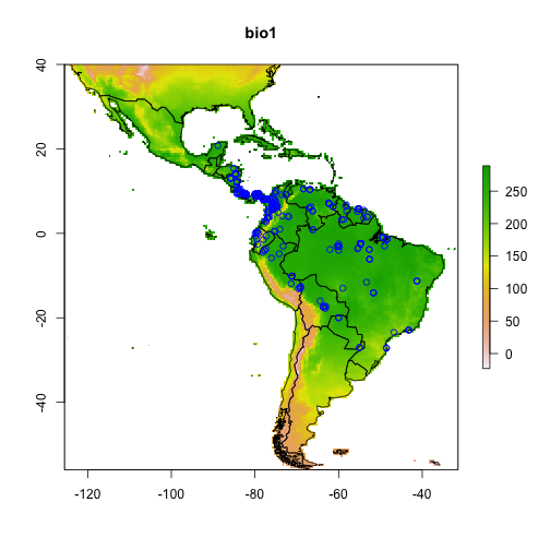
In this example, we plot actual occurrence data for Bradypus species against a single predictor variable, BIO1 (annual mean temperature). This is only ont step in a species distribution modelling nworkflow.

This example can be done using BISON data as well with our rbison package.

Load libraries

library("rgbif")
library("dismo")
library("maptools")

Raster files

Make a list of files that are installed with the dismo package, then create a rasterStack from these

files <- list.files(paste(system.file(package = "dismo"), "/ex", sep = ""), "grd", full.names = TRUE)
predictors <- stack(files)

Get world boundaries

data(wrld_simpl)

Get GBIF data using the rOpenSci package rgbif

nn <- name_lookup("bradypus*", rank = "species")
nn <- unique(nn$data$nubKey)
nn <- na.omit(nn)
df <- occ_search(taxonKey = nn, hasCoordinate = TRUE, limit = 500, return = "data")
df <- df[sapply(df, class) %in% "data.frame"]  # remove those w/o data
library("plyr")
df <- ldply(df)
df2 <- df[, c("decimalLongitude", "decimalLatitude")]

Plot

(1) Add raster data, (2) Add political boundaries, (3) Add the points (occurrences) plot(predictors, 1) plot(wrld_simpl, add = TRUE) points(df2, col = “blue”)

Further reading

The above example comes from this tutorial on species distribution modeling.