Macroecology - testing the species-abundance distribution

Keep in mind that BISON data is at least in part within GBIF, which can be accessed from R using our rgbif package. However, BISON provides a slightly different interface to their data than does GBIF, and if you are just interested in US data, then BISON may be easier to use.

In addition, this example can be done using GBIF data via rgbif.

In this example, we do some preliminary work in exploring species-abundance distribution.

Make sure to update to the latest version of rbison

Load libraries

library("rbison")
library("ggplot2")
library("plyr")

Get BISON data using the rOpenSci package rbison.

We’ll not restrain our search to any particular taxonomic group, although you will likely do that in your own research.

mynames <- c("Helianthus annuus", "Pinus contorta", "Poa annua", "Madia sativa","Arctostaphylos glauca", "Heteromeles arbutifolia", "Symphoricarpos albus","Ribes viburnifolium", "Diplacus aurantiacus", "Salvia leucophylla", "Encelia californica","Ribes indecorum", "Ribes malvaceum", "Cercocarpus betuloides", "Penstemon spectabilis")

Get data

Define a function to get data needed, here just the summary data, then pull out just the total column and make a data.frame along with the input taxon name

getdata <- function(x) {
    tmp <- bison(species = x, what = "summary")$summary
    data.frame(x, abd = tmp$total)
}

Get the data by passing each name to the getdata() function

out <- ldply(mynames, getdata)

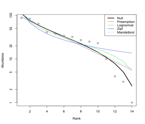
Plot

Plot species-abundance distributions using the radfit function in vegan

library(vegan)
plot(radfit(out$abd))

Further reading

Read more about plotting abundance distributions here.