Comparing occurrence data for valley oaks
rOpenSci package: rgbif
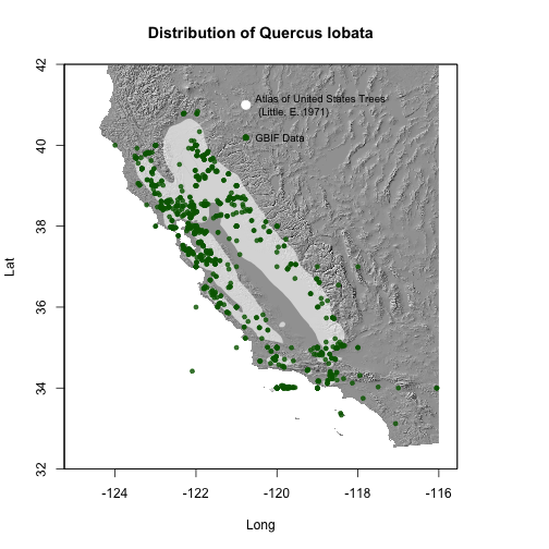
This example comes from Antonio J. Perez-Luque who shared his plot on Twitter. Antonio compared the occurrences of Valley Oak (Quercus lobata) from GBIF to the distribution of the same species from the Atlas of US Trees.
Load libraries
library('rgbif')
library('raster')
library('sp')
library('maptools')
library('rgeos')
library('scales')
Get GBIF Data for Quercus lobata
keyQl <- name_backbone(name='Quercus lobata', kingdom='plants')$speciesKey
dat.Ql <- occ_search(taxonKey=keyQl, return='data', limit=50000)
Get Distribution map of Q. lobata Atlas of US Trees (Little, E.)
From https://esp.cr.usgs.gov/data/little/. And save shapefile in same directory
url <- 'https://esp.cr.usgs.gov/data/little/querloba.zip'
tmp <- tempdir()
download.file(url, destfile = "~/querloba.zip")
unzip("~/querloba.zip", exdir = "querloba")
ql <- readShapePoly("~/querloba/querloba.shp")
Get Elevation data of US
alt.USA <- getData('alt', country='USA')
Create Hillshade of US
alt.USA <- alt.USA[[1]]
slope.USA <- terrain(alt.USA, opt='slope')
aspect.USA <- terrain(alt.USA, opt='aspect')
hill.USA <- hillShade(slope.USA, aspect.USA, angle=45, direction=315)
Plot map
plot(hill.USA, col=grey(0:100/100), legend=FALSE, xlim=c(-125,-116), ylim=c(32,42), main='Distribution of Quercus lobata', xlab="Long", ylab='Lat')
# add shape from Atlas of US Trees
plot(ql, add=TRUE, col=alpha("white", 0.6), border=FALSE)
# add Gbif presence points
points(dat.Ql$decimalLongitude, dat.Ql$decimalLatitude, cex=.7, pch=19, col=alpha("darkgreen", 0.8))
legend(x=-121, y=40.5, "GBIF Data", pch=19, col='darkgreen', bty='n', pt.cex=1, cex=.8)
legend(x=-121, y=41.5, "Atlas of United States Trees \n (Little, E. 1971)", pt.cex=1.5, cex=.8, pch=19, col='white', bty='n')