mapr tutorial
for v0.3.4
Utilities for ‘vizualizing’ species occurrence data. Includes functions to ‘vizualize’ occurrence data from ‘spocc’, ‘rgbif’, and other packages. Mapping options included for base R plots, ‘ggplot2’, and various interactive maps.
Installation
Stable version from CRAN
install.packages("mapr")
Development version from GitHub
if (!require("devtools")) install.packages("devtools")
devtools::install_github("ropensci/mapr")
library("mapr")
library("spocc")
Interactive maps
Leaflet.js
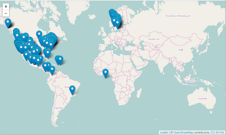
Leaflet JS is an open source mapping library that can leverage various layers from multiple sources. Using the leaflet library, we can generate a local interactive map of species occurrence data.
An example:
spp <- c('Danaus plexippus','Accipiter striatus','Pinus contorta')
dat <- occ(query = spp, from = 'gbif', has_coords = TRUE, limit = 100)
map_leaflet(dat)
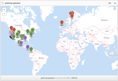
Geojson map as a Github gist
You can also create interactive maps via the mapgist function. You have to have a Github account to use this function. Github accounts are free though, and great for versioning and collaborating on code or papers. When you run the map_gist function it will ask for your Github username and password. You can alternatively store those in your .Rprofile file by adding entries for username (options(github.username = 'username')) and password (options(github.password = 'password')).
spp <- c('Danaus plexippus', 'Accipiter striatus', 'Pinus contorta')
dat <- occ(query = spp, from = 'gbif', has_coords = TRUE, limit = 100)
dat <- fixnames(dat)
map_gist(dat, color = c("#976AAE", "#6B944D", "#BD5945"))
Static maps
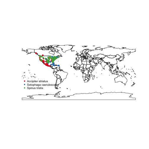
base plots
Base plots, or the built in plotting facility in R accessed via plot(), is quite fast, but not easy or efficient to use, but are good for a quick glance at some data.
spnames <- c('Accipiter striatus', 'Setophaga caerulescens', 'Spinus tristis')
out <- occ(query = spnames, from = 'gbif', has_coords = TRUE, limit = 100)
map_plot(out, size = 1, pch = 10)
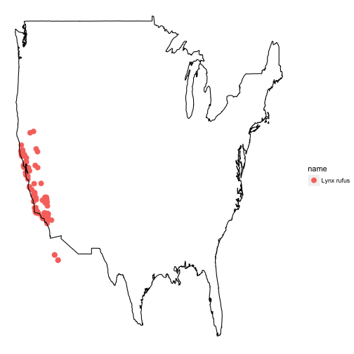
ggplot2
ggplot2 is a powerful package for making visualizations in R. Read more about it here.
dat <- occ(query = 'Lynx rufus californicus', from = 'gbif', has_coords = TRUE, limit = 200)
map_ggplot(dat, map = "usa")
Supported inputs
All functions take the following kinds of inputs:
- An object of class
occdat, from the packagespocc. An object of this class is composed of many objects of classoccdatind - An object of class
occdatind, from the packagespocc - An object of class
gbif, from the packagergbif - An object of class
data.frame. This data.frame can have any columns, but must include a column for taxonomic names (e.g.,name), and for latitude and longitude (we guess your lat/long columns, starting with the defaultlatitudeandlongitude). - An object of class
SpatialPoints - An object of class
SpatialPointsDatFrame
Citing
Scott Chamberlain (2017). mapr: ‘Visualize’ Species Occurrence Data. R package version 0.3.4. https://cran.rstudio.com/package=mapr
License and bugs
- License: MIT
- Report bugs at our GitHub repo for mapr
