magick vignette

The new magick package is an ambitious effort to modernize and simplify high-quality image processing in R. It wraps the ImageMagick STL which is perhaps the most comprehensive open-source image processing library available today.

The ImageMagick library has an overwhelming amount of functionality. The current version of Magick exposes a decent chunk of it, but being a first release, documentation is still sparse. This post briefly introduces the most important concepts to get started.

Installation

On Windows or OS-X the package is most easily installed via CRAN.

install.packages("magick")

The binary CRAN packages work out of the box and have most important features enabled. Use magick_config to see which features and formats are supported by your version of ImageMagick.

str(magick::magick_config())

#> List of 21
#>  $ version           :Class 'numeric_version'  hidden list of 1
#>   ..$ : int [1:4] 6 9 9 18
#>  $ modules           : logi FALSE
#>  $ cairo             : logi TRUE
#>  $ fontconfig        : logi TRUE
#>  $ freetype          : logi TRUE
#>  $ fftw              : logi TRUE
#>  $ ghostscript       : logi FALSE
#>  $ jpeg              : logi TRUE
#>  $ lcms              : logi FALSE
#>  $ libopenjp2        : logi FALSE
#>  $ lzma              : logi TRUE
#>  $ pangocairo        : logi TRUE
#>  $ pango             : logi TRUE
#>  $ png               : logi TRUE
#>  $ rsvg              : logi TRUE
#>  $ tiff              : logi TRUE
#>  $ webp              : logi TRUE
#>  $ wmf               : logi FALSE
#>  $ x11               : logi FALSE
#>  $ xml               : logi TRUE
#>  $ zero-configuration: logi TRUE

Image IO

What makes magick so magical is that it automatically converts and renders all common image formats. ImageMagick supports dozens of formats and automatically detects the type. Use magick::magick_config() to list the formats that your version of ImageMagick supports.

Read and write

Images can be read directly from a file path, URL, or raw vector with image data with image_read. The image_info function shows some meta data about the image, similar to the imagemagick identify command line utility.

library(magick)
tiger <- image_read('http://jeroen.github.io/images/tiger.svg')
image_info(tiger)

#>   format width height colorspace filesize
#> 1    SVG   900    900       sRGB    68630

We use image_write to export an image in any format to a file on disk, or in memory if path = NULL.

# Render svg to png bitmap
image_write(tiger, path = "tiger.png", format = "png")

If path is a filename, image_write returns path on success such that the result can be piped into function taking a file path.

Converting formats

Magick keeps the image in memory in it’s original format. Specify the format parameter image_write to convert to another format. You can also internally convert the image to another format earlier, before applying transformations. This can be useful if your original format is lossy.

tiger_png <- image_convert(tiger, "png")
image_info(tiger_png)

#>   format width height colorspace filesize
#> 1    PNG   900    900       sRGB        0

Note that size is currently 0 because ImageMagick is lazy (in the good sense) and does not render until it has to.

Preview

IDE’s with a built-in web browser (such as RStudio) automatically display magick images in the viewer. This results in a neat interactive image editing environment.

Alternatively, on Linux you can use image_display to preview the image in an X11 window. Finally image_browse opens the image in your system’s default application for a given type.

# X11 only
image_display(tiger)

# System dependent
image_browse(tiger)

Another method is converting the image to a raster object and plot it on R’s graphics display. However this is very slow and only useful in combination with other plotting functionality. See #raster below.

Transformations

The best way to get a sense of available transformations is walk through the examples in the ?transformations help page in RStudio. Below a few examples to get a sense of what is possible.

Cut and edit

Several of the transformation functions take an geometry parameter which requires a special syntax of the form AxB+C+D where each element is optional. Some examples:

• image_crop(image, "100x150+50"): crop out width:100px and height:150px starting +50px from the left
• image_scale(image, "200"): resize proportionally to width: 200px
• image_scale(image, "x200"): resize proportionally to height: 200px
• image_fill(image, "blue", "+100+200"): flood fill with blue starting at the point at x:100, y:200
• image_border(frink, "red", "20x10"): adds a border of 20px left+right and 10px top+bottom

The full syntax is specified in the Magick::Geometry documentation.

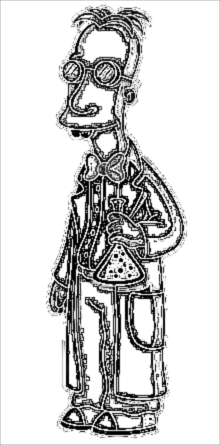
# Example image
frink <- image_read("https://jeroen.github.io/images/frink.png")
print(frink)

# Add 20px left/right and 10px top/bottom
image_border(image_background(frink, "hotpink"), "#000080", "20x10")

# Trim margins
image_trim(frink)

# Passport pica
image_crop(frink, "100x150+50")

# Resize
image_scale(frink, "300") # width: 300px

image_scale(frink, "x300") # height: 300px

# Rotate or mirror
image_rotate(frink, 45)

image_flip(frink)

image_flop(frink)

# Paint the shirt orange
image_fill(frink, "orange", point = "+100+200", fuzz = 30000)

With image_fill we can flood fill starting at pixel point. The fuzz parameter allows for the fill to cross for adjecent pixels with similarish colors. Its value must be between 0 and 256^2 specifying the max geometric distance between colors to be considered equal. Here we give professor frink an orange shirt for the World Cup.

Filters and effects

ImageMagick also has a bunch of standard effects that are worth checking out.

# Add randomness
image_blur(frink, 10, 5)

image_noise(frink)

# Silly filters
image_charcoal(frink)

image_oilpaint(frink)

image_negate(frink)

Text annotation

Finally it can be useful to print some text on top of images:

# Add some text
image_annotate(frink, "I like R!", size = 70, gravity = "southwest", color = "green")

# Customize text
image_annotate(frink, "CONFIDENTIAL", size = 30, color = "red", boxcolor = "pink",
  degrees = 60, location = "+50+100")

# Only works if ImageMagick has fontconfig
try(image_annotate(frink, "The quick brown fox", font = 'times-new-roman', size = 30), silent = T)

If your system has difficulty finding a font, you can also specify the full path to the font file in the font parameter.

Combining with pipes

Each of the image transformation functions returns a modified copy of the original image. It does not affect the original image.

frink <- image_read("https://jeroen.github.io/images/frink.png")
frink2 <- image_scale(frink, "100")
image_info(frink)

#>   format width height colorspace filesize
#> 1    PNG   220    445       sRGB    73494

image_info(frink2)

#>   format width height colorspace filesize
#> 1    PNG   100    202       sRGB        0

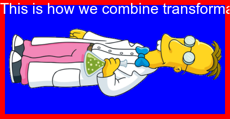
Hence to combine transformations you need to chain them:

test <- image_rotate(frink, 90)
test <- image_background(test, "blue", flatten = TRUE)
test <- image_border(test, "red", "10x10")
test <- image_annotate(test, "This is how we combine transformations", color = "white", size = 30)
print(test)

Using magrittr pipe syntax makes it a bit more readable

image_read("https://jeroen.github.io/images/frink.png") %>%
  image_rotate(270) %>%
  image_background("blue", flatten = TRUE) %>%
  image_border("red", "10x10") %>%
  image_annotate("The same thing with pipes", color = "white", size = 30)

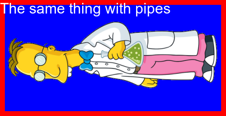
Image Vectors

The examples above concern single images. However all functions in magick have been vectorized to support working with layers, compositions or animation.

The standard base methods [ [[, c() and length() are used to manipulate vectors of images which can then be treated as layers or frames.

earth <- image_read("https://jeroen.github.io/images/earth.gif")
earth <- image_scale(earth, "200")
length(earth)

#> [1] 44

head(image_info(earth))

#>   format width height colorspace filesize
#> 1    GIF   200    200       sRGB        0
#> 2    GIF   200    200       sRGB        0
#> 3    GIF   200    200       sRGB        0
#> 4    GIF   200    200       sRGB        0
#> 5    GIF   200    200       sRGB        0
#> 6    GIF   200    200       sRGB        0

print(earth)

rev(earth) %>%
  image_flip() %>%
  image_annotate("meanwhile in Australia", size = 20, color = "white")

Layers

We can stack layers on top of each other as we would in Photoshop:

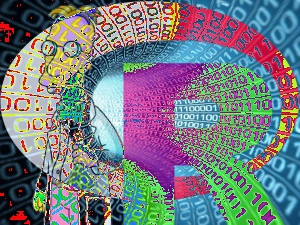
bigdata <- image_read('https://jeroen.github.io/images/bigdata.jpg')
frink <- image_read("https://jeroen.github.io/images/frink.png")
logo <- image_read("https://www.r-project.org/logo/Rlogo.png")
img <- c(bigdata, logo, frink)
img <- image_scale(img, "300x300")
image_info(img)

#>   format width height colorspace filesize
#> 1   JPEG   300    225       sRGB        0
#> 2    PNG   300    232       sRGB        0
#> 3    PNG   148    300       sRGB        0

A mosaic prints images on top of one another, expanding the output canvas such that that everything fits:

image_mosaic(img)

Flattening combines the layers into a single image which has the size of the first image:

image_flatten(img)

Flattening and mosaic allow for specifying alternative composite operators:

image_flatten(img, 'Add')

image_flatten(img, 'Modulate')

image_flatten(img, 'Minus')

Combining

Appending means simply putting the frames next to each other:

left_to_right <- image_append(image_scale(img, "x200"))
image_background(left_to_right, "white", flatten = TRUE)

Use stack = TRUE to position them on top of each other:

top_to_bottom <- image_append(image_scale(img, "100"), stack = TRUE)
image_background(top_to_bottom, "white", flatten = TRUE)

Composing allows for combining two images on a specific position:

bigdatafrink <- image_scale(image_rotate(image_background(frink, "none"), 300), "x200")
image_composite(image_scale(bigdata, "x400"), bigdatafrink, offset = "+180+100")

Pages

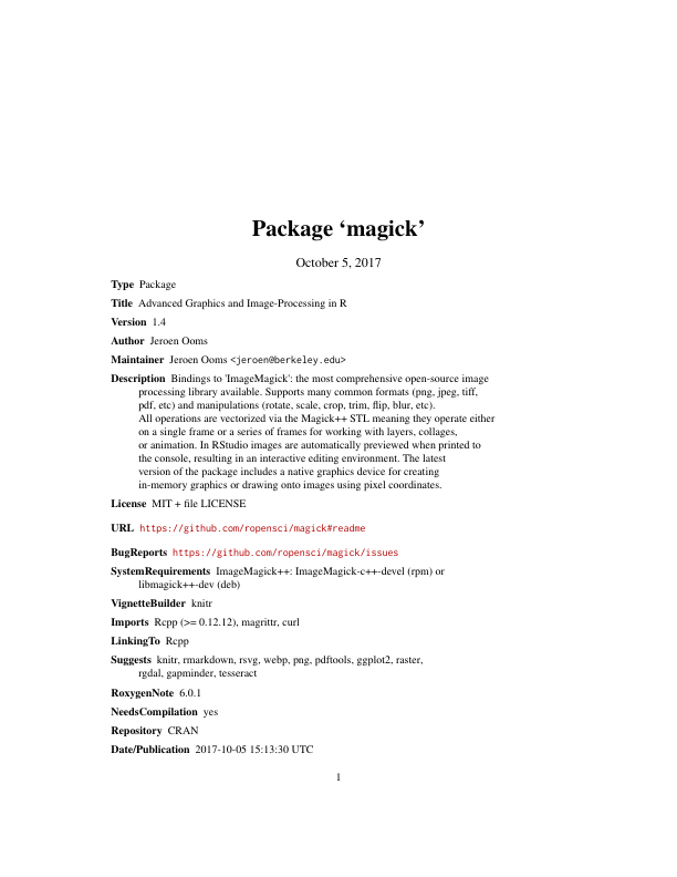
When reading a PDF document, each page becomes an element of the vector. Note that PDF gets rendered while reading so you need to specify the density immediately.

manual <- image_read('https://cran.r-project.org/web/packages/magick/magick.pdf', density = "72x72")
image_info(manual)

# Convert the first page to PNG
image_convert(manual[1], "png", 8)

Magick requires ghostscript to render the PDF. An alternative method to read pdf is render it via the pdftools package:

library(pdftools)
bitmap <- pdf_render_page('https://cran.r-project.org/web/packages/magick/magick.pdf',
  page = 1, dpi = 72, numeric = FALSE)
image_read(bitmap)

Animation

Instead of treating vector elements as layers, we can also make them frames in an animation!

image_animate(image_scale(img, "200x200"), fps = 1, dispose = "previous")

Morphing creates a sequence of n images that gradually morph one image into another. It makes animations

newlogo <- image_scale(image_read("https://www.r-project.org/logo/Rlogo.png"), "x150")
oldlogo <- image_scale(image_read("https://developer.r-project.org/Logo/Rlogo-3.png"), "x150")
frames <- image_morph(c(oldlogo, newlogo), frames = 10)
image_animate(frames)

If you read in an existing GIF or Video file, each frame becomes a layer:

# Foreground image
banana <- image_read("https://jeroen.github.io/images/banana.gif")
banana <- image_scale(banana, "150")
image_info(banana)

#>   format width height colorspace filesize
#> 1    GIF   150    148       sRGB        0
#> 2    GIF   150    148       sRGB        0
#> 3    GIF   150    148       sRGB        0
#> 4    GIF   150    148       sRGB        0
#> 5    GIF   150    148       sRGB        0
#> 6    GIF   150    148       sRGB        0
#> 7    GIF   150    148       sRGB        0
#> 8    GIF   150    148       sRGB        0

Manipulate the individual frames and put them back into an animation:

# Background image
background <- image_background(image_scale(logo, "200"), "white", flatten = TRUE)

# Combine and flatten frames
frames <- image_apply(banana, function(frame) {
  image_composite(background, frame, offset = "+70+30")
})

# Turn frames into animation
animation <- image_animate(frames, fps = 10)
print(animation)

Animations can be saved as GIF of MPEG files:

image_write(animation, "Rlogo-banana.gif")

Drawing and Graphics

A relatively recent addition to the package is a native R graphics device which produces a magick image object. This can either be used like a regular device for making plots, or alternatively to open a device which draws onto an existing image using pixel coordinates.

Graphics device

The image_graph() function opens a new graphics device similar to e.g. png() or x11(). It returns an image objec to which the plot(s) will be written. Each “page” in the plotting device will become a frame in the image object.

# Produce image using graphics device
fig <- image_graph(width = 400, height = 400, res = 96)
ggplot2::qplot(mpg, wt, data = mtcars, colour = cyl)
dev.off()

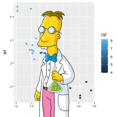
We can easily postprocess the figure using regular image operations.

# Combine
out <- image_composite(fig, frink, offset = "+70+30")
print(out)

Drawing device

Another way to use the graphics device is to draw on top of an exiting image using pixel coordinates.

# Or paint over an existing image
img <- image_draw(frink)
rect(20, 20, 200, 100, border = "red", lty = "dashed", lwd = 5)
abline(h = 300, col = 'blue', lwd = '10', lty = "dotted")
text(30, 250, "Hoiven-Glaven", family = "courier", cex = 4, srt = 90)
palette(rainbow(11, end = 0.9))
symbols(rep(200, 11), seq(0, 400, 40), circles = runif(11, 5, 35),
  bg = 1:11, inches = FALSE, add = TRUE)
dev.off()

print(img)

By default image_draw() sets all margins to 0 and uses graphics coordinates to match image size in pixels (width x height) where (0,0) is the top left corner. Note that this means the y axis increases from top to bottom which is the opposite of typical graphics coordinates. You can override all this by passing custom xlim, ylim or mar values to image_draw.

Animated Graphics

The graphics device supports multiple frames which makes it easy to create animated graphics. The code below shows how you would implement the example from the very cool gganimate package using the magick graphics device.

library(gapminder)
library(ggplot2)
img <- image_graph(600, 400, res = 96)
datalist <- split(gapminder, gapminder$year)
out <- lapply(datalist, function(data){
  p <- ggplot(data, aes(gdpPercap, lifeExp, size = pop, color = continent)) +
    scale_size("population", limits = range(gapminder$pop)) + geom_point() + ylim(20, 90) +
    scale_x_log10(limits = range(gapminder$gdpPercap)) + ggtitle(data$year) + theme_classic()
  print(p)
})
dev.off()
img <- image_background(image_trim(img), 'white')
animation <- image_animate(img, fps = 2)
print(animation)

To write it to a file you would simply do:

image_write(animation, "gapminder.gif")

Raster Images

Magick images can also be converted to raster objects for use with R’s graphics device. Thereby we can combine it with other graphics tools. However do note that R’s graphics device is very slow and has a very different coordinate system which reduces the quality of the image.

Base R rasters

Base R has an as.raster format which converts the image to a vector of strings. The paper Raster Images in R Graphics by Paul Murrell gives a nice overview.

plot(as.raster(frink))

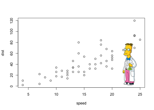
# Print over another graphic
plot(cars)
rasterImage(frink, 21, 0, 25, 80)

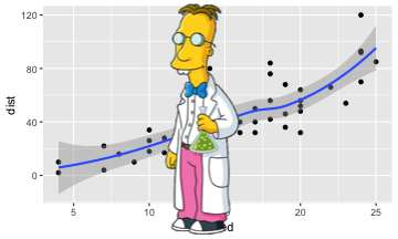
The grid package

The grid package makes it easier to overlay a raster on the graphics device without having to adjust for the x/y coordinates of the plot.

library(ggplot2)
library(grid)
qplot(speed, dist, data = cars, geom = c("point", "smooth"))
grid.raster(frink)

The raster package

The raster package has it’s own classes for bitmaps which are useful for spatial applications. The simplest way to convert an image to raster is export it as a tiff file:

tiff_file <- tempfile()
image_write(frink, path = tiff_file, format = 'tiff')
r <- raster::brick(tiff_file)
raster::plotRGB(r)

You can also manually convert the bitmap array into a raster object, but this seems to drop some meta data:

buf <- as.integer(frink[[1]])
rr <- raster::brick(buf)
raster::plotRGB(rr, asp = 1)

The raster package also does not seem to support transparency, which perhaps makes sense in the context of spatial imaging.

OCR text extraction

A recent edition to the package is to extract text from images using OCR. This requires the tesseract package:

install.packages("tesseract")

img <- image_read("http://jeroen.github.io/images/testocr.png")
print(img)

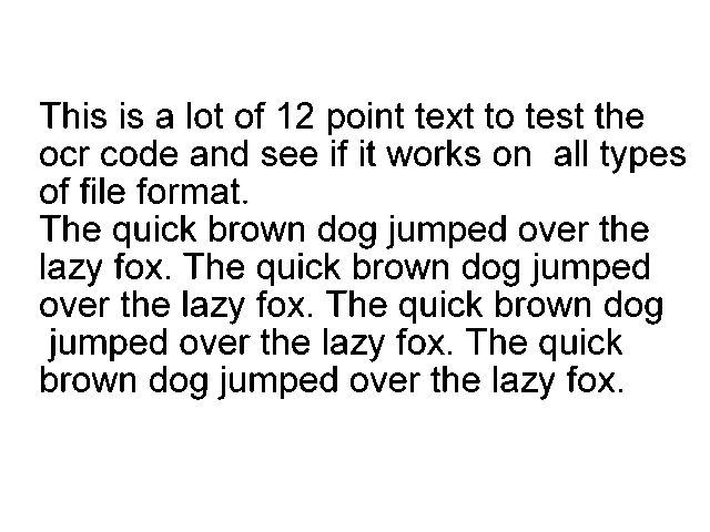
# Extract text
cat(image_ocr(img))

#> This is a lot of 12 point text to test the
#> cor code and see if it works on all types
#> of file format.
#>
#> The quick brown dog jumped over the
#> lazy fox. The quick brown dog jumped
#> over the lazy fox. The quick brown dog
#> jumped over the lazy fox. The quick
#> brown dog jumped over the lazy fox.

Citing

Jeroen Ooms (2017). magick: Advanced Graphics and Image-Processing in R. R package version 1.4. https://CRAN.R-project.org/package=magick

License and bugs

• License: MIT
• Report bugs at our GitHub repo for magick

Back to top