gender tutorial
for v0.5.1
gender encodes gender based on names and dates of birth using historical datasets. By using these datasets instead of lists of male and female names, this package is able to more accurately guess the gender of a name, and it is able to report the probability that a name was male or female.
Installation
install.packages("gender")
Or development version from GitHub
devtools::install_github("ropensci/gender")
library("gender")
Usage
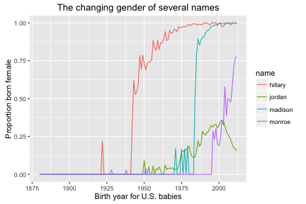
A common problem for researchers who work with data, especially historians, is that a dataset has a list of people with names but does not identify the gender of the person. Since first names often indicate gender, it should be possible to predict gender using names. However, the gender associated with names can change over time. To illustrate, take the names Madison, Hillary, Jordan, and Monroe. For babies born in the United States, those predominant gender associated with those names has changed over time.
Predicting gender from names requires a fundamentally historical method. The gender package provides a way to calculate the proportion of male and female names given a year or range of birth years and a country or set of countries. The predictions are based on calculations from historical datasets.
This vignette offers a brief guide to the gender package. For a fuller historical explanation and a sample case study using the package, please see our journal article: Cameron Blevins and Lincoln Mullen, “Jane, John … Leslie? A Historical Method for Algorithmic Gender Prediction,” Digital Humanities Quarterly (forthcoming 2015).
Basic usage
The main function in this package is gender(). That function lets you choose a dataset and pass in a set of names and a birth year or range of birth years. The result is always a data frame that includes a prediction of the gender of the name and the relative proportions between male and female. For example:
library(gender)
gender(c("Madison", "Hillary"), years = 1940, method = "demo")
#> # A tibble: 2 x 6
#>      name proportion_male proportion_female gender year_min year_max
#>     <chr>           <dbl>             <dbl>  <chr>    <dbl>    <dbl>
#> 1 Hillary               1                 0   male     1940     1940
#> 2 Madison               1                 0   male     1940     1940
gender(c("Madison", "Hillary"), years = 2000, method = "demo")
#> # A tibble: 2 x 6
#>      name proportion_male proportion_female gender year_min year_max
#>     <chr>           <dbl>             <dbl>  <chr>    <dbl>    <dbl>
#> 1 Hillary          0.0000            1.0000 female     2000     2000
#> 2 Madison          0.0069            0.9931 female     2000     2000
The gender package itself contains only demonstration data. Datasets which permit you to make predictions for various times and places are available in the genderdata package. This package is not available on CRAN because of its size. The first time that you need to use the dataset you will be prompted to install it, or you can install it yourself from the rOpenSci repository:
install.packages("genderdata", repos = "http://packages.ropensci.org")
You specify which dataset you wish to use with the method = parameter. Below are some sample
United States in the 1960s:
gender("Madison", years = c(1960, 1969), method = "ssa")
United States in the 1860s:
gender("Madison", years = c(1860, 1869), method = "ipums")
North Atlantic countries in the 1860s:
gender("Hilde", years = c(1860, 1869), method = "napp")
Just Sweden in the 1879:
gender("Hilde", years = c(1879), method = "napp", countries = "Sweden")
Which dataset should you use?
Each method is associated with a dataset suitable for a particular time and place.
method = "ipums": United States from 1789 to 1930. Drawn from Census data.method = "ssa": United States from 1930 to 2012. Drawn from Social Security Administration data.method = "napp": Any combination of Canada, the United Kingdom, Germany, Iceland, Norway, and Sweden from the years 1758 to 1910, though the nineteenth-century data is likely more reliable than the eighteenth-century data.
Description of the datasets
U.S. Census data is provided by IPUMS USA from the Minnesota Population Center, University of Minnesota. The IPUMS data includes 1% and 5% samples from the Census returns. The Census, taken decennially, includes respondent’s birth dates and gender. With the gender package, it is possible to use this dataset for years between 1789 and 1930. The dataset includes approximately 339,967 unique names.
U.S. Social Security Administration data was collected from applicants to Social Security. The Social Security Board was created in the New Deal in 1935. Early applicants, however, were people who were nearing retirement age not people who were being born, so the dataset extends further into the past. However, the Social Security Administration did not immediately require all persons born in the United States to register for a Social Security Number. (See Shane Landrum, “The State’s Big Family Bible: Birth Certificates, Personal Identity, and Citizenship in the United States, 1840–1950” [PhD dissertation, Brandeis University, 2014].) A consequence of this—for reasons that are not entirely clear—is that for years before 1918, the SSA dataset is heavily female; after about 1940 it skews slightly male. For this reason this package corrects the prediction to assume a secondary sex ratio that is evenly distributed between males and females. Also, the SSA dataset only includes names that were used more than five times in a given year, so the “long tail” of names is excluded. Even so, the dataset includes 91,320 unique names. The SSA dataset extends from 1880 to 2012, but for years before 1930 you should use the IPUMS method.
The North Atlantic Population Project provides data for Canada, the United Kingdom, Germany, Iceland, Norway, and Sweden for years between 1758 and 1910, based on census microdata from those countries.
Working with data frames of names
Most often you have a dataset and you want to predict gender for multiple names. Consider this sample dataset.
library(dplyr)

demo_names <- c("Susan", "Susan", "Madison", "Madison",
                "Hillary", "Hillary", "Hillary")
demo_years <- c(rep(c(1930, 2000), 3), 1930)
demo_df <- data_frame(first_names = demo_names,
                      last_names = LETTERS[1:7],
                      years = demo_years,
                      min_years = demo_years - 3,
                      max_years = demo_years + 3)

demo_df
#> # A tibble: 7 x 5
#>   first_names last_names years min_years max_years
#>         <chr>      <chr> <dbl>     <dbl>     <dbl>
#> 1       Susan          A  1930      1927      1933
#> 2       Susan          B  2000      1997      2003
#> 3     Madison          C  1930      1927      1933
#> 4     Madison          D  2000      1997      2003
#> 5     Hillary          E  1930      1927      1933
#> 6     Hillary          F  2000      1997      2003
#> 7     Hillary          G  1930      1927      1933
Here we have a dataset with first names connected to years. It is important to emphasize that these years should be the years of birth. If you have years representing something else, you will have to estimate the years of birth. For this demo dataset, we have included a single birth year for each person. But since historians may only have a guess at the birth year of people, we have also included columns for the minimum and maximum years in an possible age range.
We can pass this data frame to the gender_df() function, specifying the method that we wish to use and the names of the columns that contain the names and the birth years. The result is a data frame of predictions.
results <- gender_df(demo_df, name_col = "first_names", year_col = "years",
                     method = "demo")
results
#> # A tibble: 6 x 6
#>      name proportion_male proportion_female gender year_min year_max
#> *   <chr>           <dbl>             <dbl>  <chr>    <dbl>    <dbl>
#> 1 Hillary          1.0000            0.0000   male     1930     1930
#> 2 Madison          1.0000            0.0000   male     1930     1930
#> 3   Susan          0.0000            1.0000 female     1930     1930
#> 4 Hillary          0.0000            1.0000 female     2000     2000
#> 5 Madison          0.0069            0.9931 female     2000     2000
#> 6   Susan          0.0000            1.0000 female     2000     2000
Notice that in our original data frame there were two Hillarys (Hillary E and Hillary G) born in 1930, but our resulting data frame only contains one. That is because the gender_df() function is efficient, calculating genders only for unique combinations of first names and years. In a dataset of any appreciable size, this saves quite a bit of computation time. The resulting data frame can be merged back into the original dataset.
demo_df %>%
  left_join(results, by = c("first_names" = "name", "years" = "year_min"))
#> # A tibble: 7 x 9
#>   first_names last_names years min_years max_years proportion_male
#>         <chr>      <chr> <dbl>     <dbl>     <dbl>           <dbl>
#> 1       Susan          A  1930      1927      1933          0.0000
#> 2       Susan          B  2000      1997      2003          0.0000
#> 3     Madison          C  1930      1927      1933          1.0000
#> 4     Madison          D  2000      1997      2003          0.0069
#> 5     Hillary          E  1930      1927      1933          1.0000
#> 6     Hillary          F  2000      1997      2003          0.0000
#> 7     Hillary          G  1930      1927      1933          1.0000
#> # ... with 3 more variables: proportion_female <dbl>, gender <chr>,
#> #   year_max <dbl>
We can also use gender_df() to predict gender a range of years by passing it the names of columns with minimum and maximum years of the range to be used for each person. As in the previous example, only unique combinations of first names and ranges of years will be calculated.
gender_df(demo_df, name_col = "first_names",
          year_col = c("min_years", "max_years"), method = "demo")
#> # A tibble: 6 x 6
#>      name proportion_male proportion_female gender year_min year_max
#> *   <chr>           <dbl>             <dbl>  <chr>    <dbl>    <dbl>
#> 1 Hillary          1.0000            0.0000   male     1927     1933
#> 2 Madison          1.0000            0.0000   male     1927     1933
#> 3   Susan          0.0028            0.9972 female     1927     1933
#> 4 Hillary          0.0092            0.9908 female     1997     2003
#> 5 Madison          0.0081            0.9919 female     1997     2003
#> 6   Susan          0.0000            1.0000 female     1997     2003
Working with dplyr
The gender_df() function is simply a wrapper around a dplyr data manipulation chain. Should you wish, you can use dplyr’s do() function to run the gender() function on each name and birth year (i.e., each row). This will result in a dataframe containing a column of dataframes. Another call to do() and bind_rows() will create a the single data frame that we expect.
demo_df %>%
  distinct(first_names, years) %>%
  rowwise() %>%
  do(results = gender(.$first_names, years = .$years, method = "demo")) %>%
  do(bind_rows(.$results))
#> Source: local data frame [6 x 6]
#> Groups: <by row>
#>
#> # A tibble: 6 x 6
#>      name proportion_male proportion_female gender year_min year_max
#> *   <chr>           <dbl>             <dbl>  <chr>    <dbl>    <dbl>
#> 1   Susan          0.0000            1.0000 female     1930     1930
#> 2   Susan          0.0000            1.0000 female     2000     2000
#> 3 Madison          1.0000            0.0000   male     1930     1930
#> 4 Madison          0.0069            0.9931 female     2000     2000
#> 5 Hillary          1.0000            0.0000   male     1930     1930
#> 6 Hillary          0.0000            1.0000 female     2000     2000
That method of using dplyr is the most intuitive, since it calls gender() once for each row. (In the example above, there are six calls to the function.) However, because of the way that the gender() function works, it can handle multiple names provided that they all use the same range of years. In other words, we will do better to group the data frame by the year. In the code below, we call gender() once for each year (i.e. two times) which results in a considerable time savings.
demo_df %>%
  distinct(first_names, years) %>%
  group_by(years) %>%
  do(results = gender(.$first_names, years = .$years[1], method = "demo")) %>%
  do(bind_rows(.$results))
#> Source: local data frame [6 x 6]
#> Groups: <by row>
#>
#> # A tibble: 6 x 6
#>      name proportion_male proportion_female gender year_min year_max
#> *   <chr>           <dbl>             <dbl>  <chr>    <dbl>    <dbl>
#> 1 Hillary          1.0000            0.0000   male     1930     1930
#> 2 Madison          1.0000            0.0000   male     1930     1930
#> 3   Susan          0.0000            1.0000 female     1930     1930
#> 4 Hillary          0.0000            1.0000 female     2000     2000
#> 5 Madison          0.0069            0.9931 female     2000     2000
#> 6   Susan          0.0000            1.0000 female     2000     2000
These results can then be joined back into your original dataset.
Citing
To cite gender in publications use:
Lincoln Mullen (2015). gender: Predict Gender from Names Using Historical Data. R package version 0.5.1 https://github.com/ropensci/gender
License and bugs
- License: MIT
- Report bugs at our Github repo for gender
